Modelling Mars’ Atmosphere for Simulating Blunt Body Entry Vehicles

(Expanded Image) This is one of the outputs of this project, a simulated entry of the Perseverance Mars rover compared to real data.

For a fun application of this model and explanation of one of the tradeoffs in designing a Mars lander and Mars lander trajectories, see the companion blog post to this one.

Here I describe how the model works, my process in creating it, and backtesting to real Mars lander data.

Links to Github and project notes.

Introduction to Modelling Mars Landers

Free body diagram of the blunt body entry vehicle used in the model.

My goal with this project was to create a minimum viable Martian atmosphere model that could be used to simulate the entry of blunt body vehicles with various parameters (drag coefficient, ballistic coefficient, angle of attack, etc.).

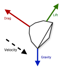
In keeping with this goal, I sought to keep the model as simple as possible. Hence, there are only three forces acting on the vehicle: drag, lift, and gravity.

I used multiple papers to determine the values for the parameters used in the model. For example, I used the paper Aerodynamics for the Mars Phoenix Entry Capsule to determine the drag coefficient vs. velocity for the Phoenix lander, and generalized this to other blunt body vehicles. All papers and sources I found are listed in the Google Doc containing my project notes.

Other data gained from papers on Mars’ atmosphere / Mars landers include:

By assuming all blunt body entry vehicles are similar, I did not have to create a complex aerothermodynamic model for each vehicle, instead using the same parameters and functions for coefficent of drag vs. velocity, etc. for all of them. I tested this hypothesis by backtesting the model against real data on various Mars landers and got encouraging results (see the chart of simulated vs. real Perseverance landing data).

See Appendix 1 for more explanation of modelling blunt body vehicles.

Finding and Implementing Martian Atmosphere Data

Getting Data From Papers

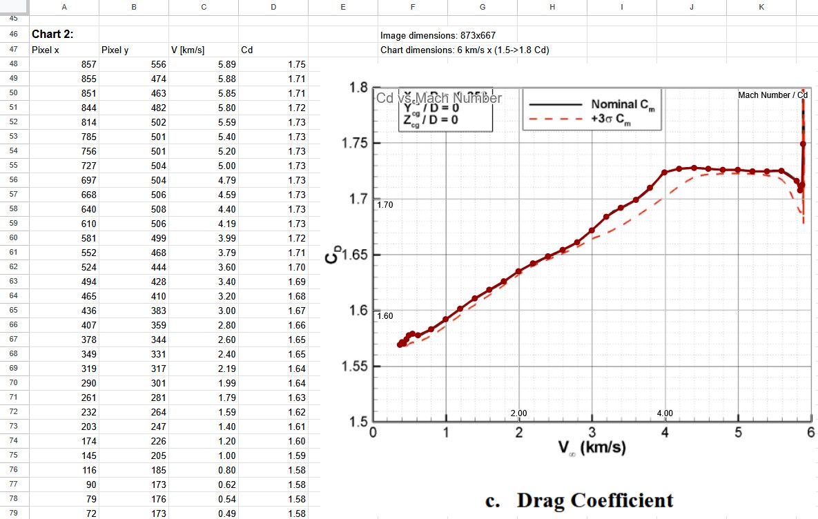
(Expanded Image) This shows translation of pixel locations on a screenshot of a chart from a paper into useful values.

Before I could begin implementing the model, I needed to find quantitative data on the Martian atmosphere in a format I could use. Unfortunately, most papers do not give you .csv’s of their data, and instead give you charts. So I resorted to pixel counting in Krita and writing Python scripts to extract data from the charts.

With the points on the various charts extracted, I used numpy to interpolate between the points to create a mostly smooth curve (eg. you can see interpolated points in the Google Sheets chart above).

Note that if you have any use for this data, it’s all found as numpy arrays on the project’s Github under utils.py.

I wrote (with the help of the LLMs) several Python scripts to automate data extraction, some of which you might find useful (available on Github):

To extract pixel positions from a line chart:
- image_point_select.py (Click on an image to add points, then get points in a list)
- line_point_extract.py (Automatically extract points from a particular colour line)
For converting pixel positions to values:
- points-to-values.py (Convert pixel positions into useful values automatically, no Google Sheets involved!)
For converting data into more useful formats:
- sheets_to_np_array.py (Convert Google Sheets values / other script output into numpy arrays)
- rebase_graph_interpolation.py (Rebase two graphs to the same x-axis, then interpolate between them to unify)
- hvel_to_downreange_dist.py (Convert horizontal velocity to downrange distance)

Atmospheric Pressure Data

(Expanded Image) NASA Website approximation of Martian atmospheric pressure (red) compared to NASA MarsGRAM (blue).

In the name of simplicity, my first approach was to approximate Mars’ atmospheric pressure with this function from a NASA website:
p = 0.699 * exp(-0.00009 * h)

However, I noticed some inconsistencies between my simulated vehicles and the real data. Particularly, in the upper atmosphere, my vehicles began decelerating too early.

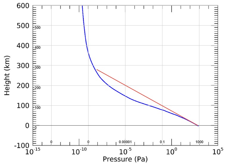
This prompted me to look for papers that show Mars’ atmospheric pressure vs. altitude. I wanted to get access to NASA’s MarsGRAM tool, but it was unavailable to me (Canada issue?). However, the user guide shows an example output of the tool, which just happens to be pressure vs. altitude.

Comparing both graphs above, we clearly see that the first approximation I used diverges in the upper atmosphere. So, more pixel counting was required to get the better data from the MarsGRAM user guide.

I later found a few other papers that also have pressure vs. altitude data. If I continue this project, it may be worth it to compare all data sources to see if they are consistent with each other.

Atmospheric Temperature Data

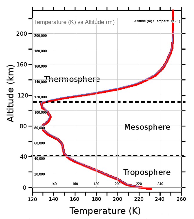
(Expanded Image) Mars Altitude vs. Temperature from this paper.

I found two papers that show Martian atmospheric temperature vs. altitude. Both agree with each other on the rough shape of the curve and the values.

Interestingly, Mars’ atmosphere is coldest around 80-120 km above the surface, then the temperature increases to a limit of ~250 K as altitude approaches infinity. Maybe this is an artifact of the temperature measurement method, or maybe it’s a real phenomenon I’ll have to learn about in the future.

Atmospheric Density Data

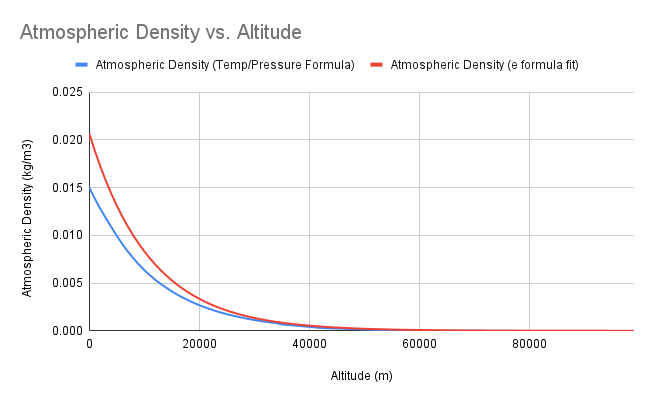
Comparing two sources for Mars’ Atmospheric Pressure. The blue line ended up giving more accurate results.

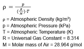
Initially, I used a formula and parameters from the NASA Mars Fact Sheet to calculate atmospheric density:

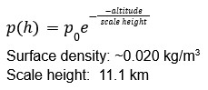
During testing against historic Mars lander data, I found that the density values were too high. Instead, I found another formula to approximate density from this NASA Website.

This results in far lower atmospheric density values than the previous formula (see the graph above). At this point, I hadn’t yet found any papers that had density vs. altitude data to compare to, though I later found a few.

Because this function is more complex than the previous one (having on pressure and temperature), to ensure all the data was in the right ballpark, I compared the values to data from the Viking landers:

Average Martian temperature is 210 K
Viking landing site pressure range: 690 to 900 Pa
Viking landing site temperature range: 184 to 242 K

Using the formula above, we get these atmospheric density values:
(P, T): Density
900, 184: 0.02546 kg/m3
690, 184: 0.01952 kg/m3
900, 242: 0.01936 kg/m3
690, 242: 0.01484 kg/m3

We’re at the low end of the Viking range with a maximum density of ~0.015 kg/m3 (See chart above). Given that the pressure data I used reaches a maximum of ~700 Pa while Viking supposedly reaches 900 Pa (Mars is apparently 600 Pa on average), I believe my values are reasonable.

Drag Coefficient and Lift-to-Drag Ratio

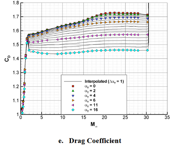
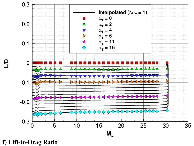
As mentioned earlier, I used the paper Aerodynamics for the Mars Phoenix Entry Capsule to find the drag coefficient vs. velocity and lift-to-drag ratio vs. angle of attack for the Phoenix lander.

I’m only now realizing that the drag coefficient vs. velocity graph is given for multiple angles of attack, and I only implemented the 0-degree AoA curve. Whoops! This results in higher than expected drag force for higher angles of attack, which I will have to fix if I continue this project.

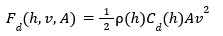
To calculate the drag force, I used this formula:

Then, I solved for lift using the lift-to-drag ratio:
(Lift/Drag Ratio) * Drag = Lift

Equations & Building The Model in Python

I used a timestep-based Newtonian physics model to simulate the vehicle’s trajectory. This model used a few basic equations to calculate the forces acting on the vehicle, then calculated acceleration, velocity, and position at each timestep.

Acceleration due to drag:

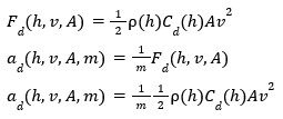
Acceleration due to gravity:

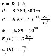
Acceleration due to lift (same as before but with acceleration instead of force as the variables):
(Lift/Drag Ratio) * Drag = Lift

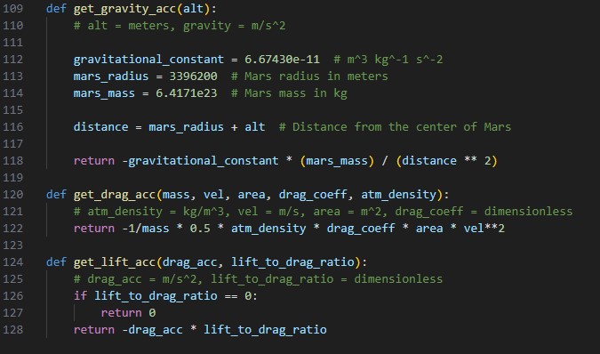Acceleration functions implemented in Python in sim.py.

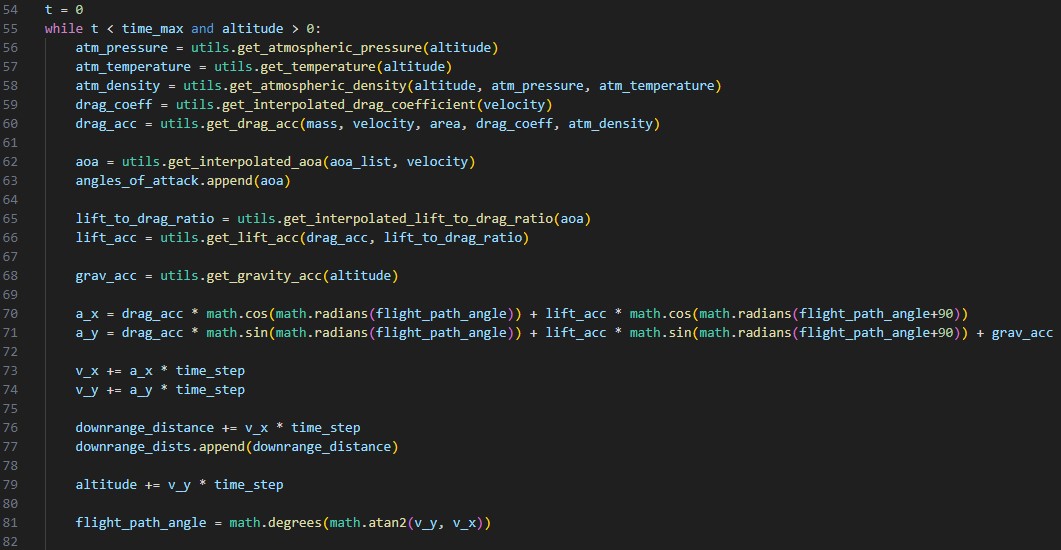Simulation time step implemented in Python in sim.py.

With each iteration of the simulation, the atmospheric pressure, temperature and density are calculated based on the current altitude.

These values are fed into the acceleration functions to calculate the drag, lift, and gravity accelerations.

Next, total acceleration is calculated using the flight path angle (the angle between the velocity vector and the horizontal plane).

Finally, velocity and position are updated and the loop continues until the vehicle impacts the surface.

Initial Simulations and Convergence as a Function of Time Step

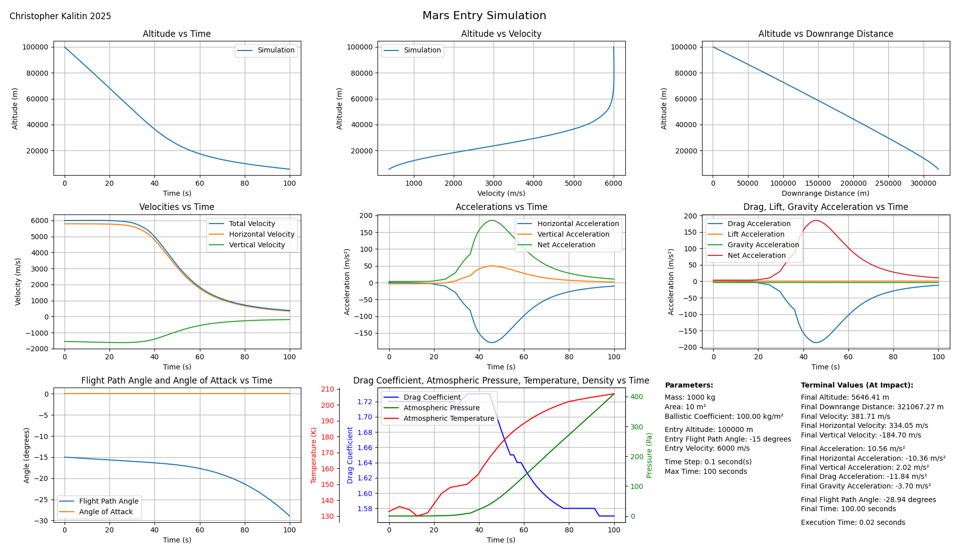
(Expanded Image) This is one of the first simulations done using the model. (Shown using updated interface so that it’s consistent with other charts in this post)

Once I had a first iteration of the model, I ran a few simulations and worked on the matplotlib interface to visualize the results.

Explanation of Subplots

Altitude vs. Time - self-explanatory
Altitude vs. Velocity - This is a standard plot used for Mars entry vehicles. On the right, we see the vehicle in the upper atmosphere while it still has high velocity. As it descends, we see how altitude and velocity decrease relative to each other.
Altitude vs. Downrange Distance - This is essentially y position vs. x position, and shows the exact trajectory of the vehicle.
Velocities vs. Time - This shows total, horizontal, and vertical velocities. Note that total velocity is the vector sum of horizontal and vertical velocity and only reflects magnitude, not direction.
Accelerations vs. Time - Just like the velocity plot, the net acceleration is the vector sum of the horizontal and vertical accelerations and only reflects the magnitude of acceleration, not the direction of net acceleration. So, don’t worry about the lack of negative values for net acceleration.
Drag, Lift, and Gravity acceleration vs. Time - Again, self-explanatory
Flight Path Angle and Angle of Attack vs. Time
- Flight Path Angle: The angle between the horizontal plane and the velocity vector.
- Angle of Attack: The angle between the vehicle’s velocity vector and the vehicle’s body axis. Essentially measures pitch/yaw.
Drag Coefficient, Atmospheric Pressure, Temperature, and Density vs. Time - Drag coefficient is a function of velocity, while atmospheric pressure, temperature, and density are functions of altitude. Here we see their exact values at each time step (you can cross-reference with the velocity or altitude plots to see how they relate to vel & alt).
Parameters - These are the initial parameters of the simulation
Terminal Values - This shows you the status of the vehicle at the end of the simulation.

Convergence as a Function of Timestep

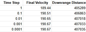
This shows simulation terminal values vs. time step size.

Because I’m using discrete time steps and not a continuous integration method, the size of the time step can affect the accuracy of the simulation. This is an inherent limitation of all numerical integration/differentiation methods.

To test what impact the time step size has on the simulation, I ran a single simulation with a varying time step and recorded the terminal values.

We can see above that there are diminishing returns to decreasing the time step size (as expected). I ended up using 0.1s as the time step for the final model and the simulations in the companion blog post as I found it to be a good balance between accuracy and simulation time.

Fitting To Opportunity

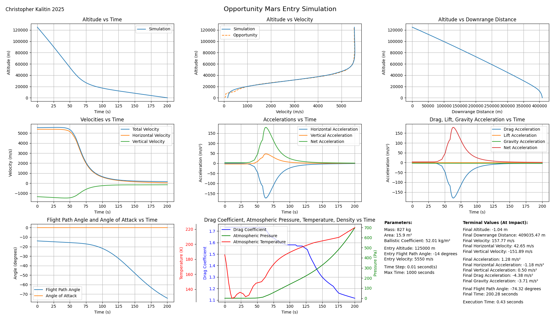
(Expanded Image) This is my simulation of the Opportunity rover’s Mars atmospheric entry.

All the explanation above of gathering Martian atmospheric data and building the model is not given in chronological order. In reality, progress was not monotonic and I had several intermediary iterations of the model before I got to the final version.

One intermediary test I did was to simulate the Opportunity rover’s entry trajectory and compare to it real data taken from chapter 9 of Casey Handmer’s How To Get To Earth From Mars.

Because Opportunity followed a ballistic trajectory on descent, it had no active control of its angle of attack and was purely a passive entry vehicle. This meant I could use it as a test case for the model before I had implemented angle of attack and lift.

The top middle chart of the image above shows the simulated vs. real altitude vs. velocity plot, and it’s remarkably close! The divergence comes when at ~600m/s the real Opportunity rover pulled its parachute, which I don’t model. Overall, great success!

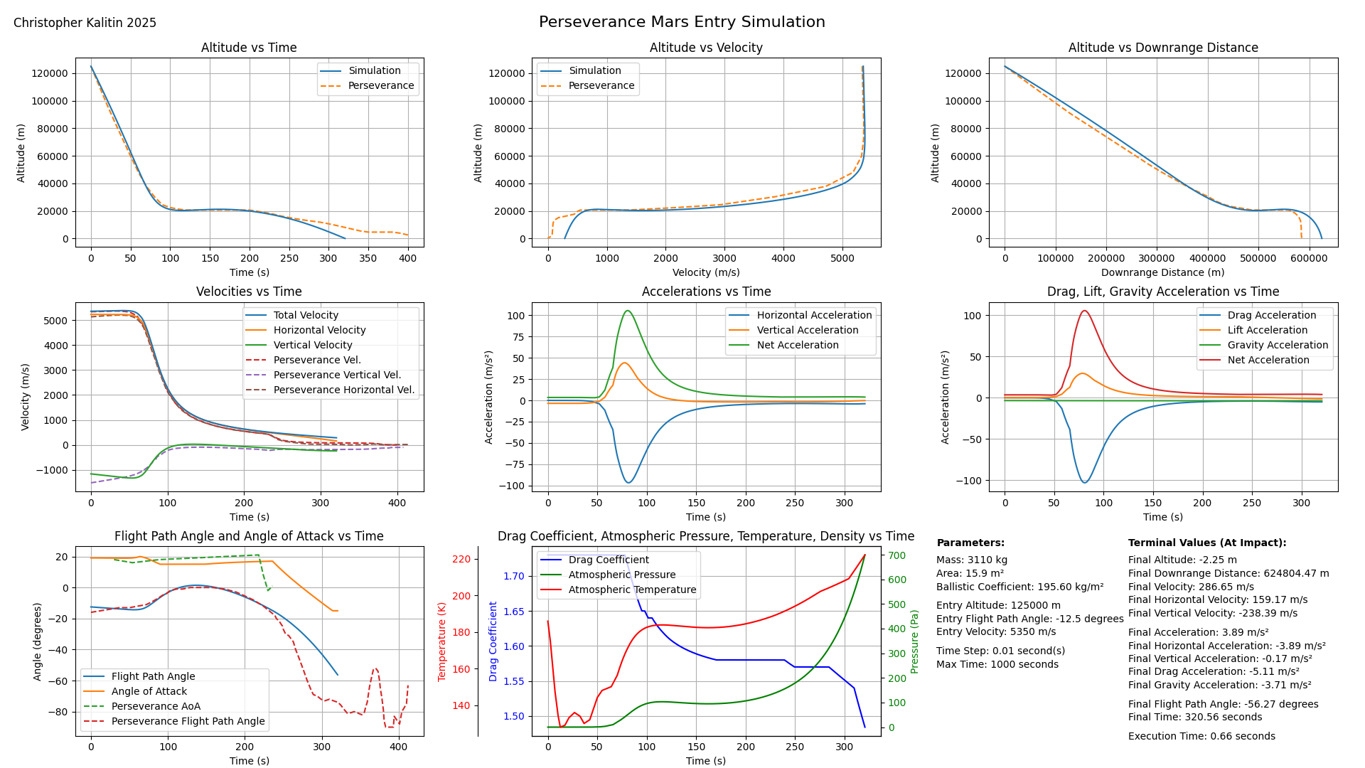
Fitting To Perseverance

(Expanded Image) This is my simulation of the Perseverance rover’s Mars atmospheric entry.

After a difficult process of just trying to find a paper that contained the Perseverance Mars entry data (See Appendix 2), I was able to extract a trove of data including altitude; net velocity; east, north, down velocities; flight path angle; angle of attack; and even more that I didn’t include.

The Perseverance entry vehicle weighs about 4x as much as Opportunity (3110 kg and 827 kg, respectively) while having the same radius (2.25 m). Because drag force is proportional to area and not mass, this means that the acceleration due to drag under the same conditions is 4x less for Perseverance than for Opportunity. Hence, if Perseverance followed the same ballistic trajectory as Opportunity, it would have a far higher velocity at the time of impact.

This is why Curiosity and Perseverance both used ~20-degree angles of attack during entry. This allows them to generate lift so that they can spend more time in the atmosphere before impact, allowing drag more time to slow them down. The bottom left chart shows simulated and real angle of attack vs. time.

Just like we saw with Opportunity, the model has a major divergence when the parachute is deployed at ~240s. Overall, the model doesn’t fit quite as well as it did for Opportunity (this may be due to overestimating the drag coefficient, mentioned above), but it fits well enough to be useful.

Fitting To Starship

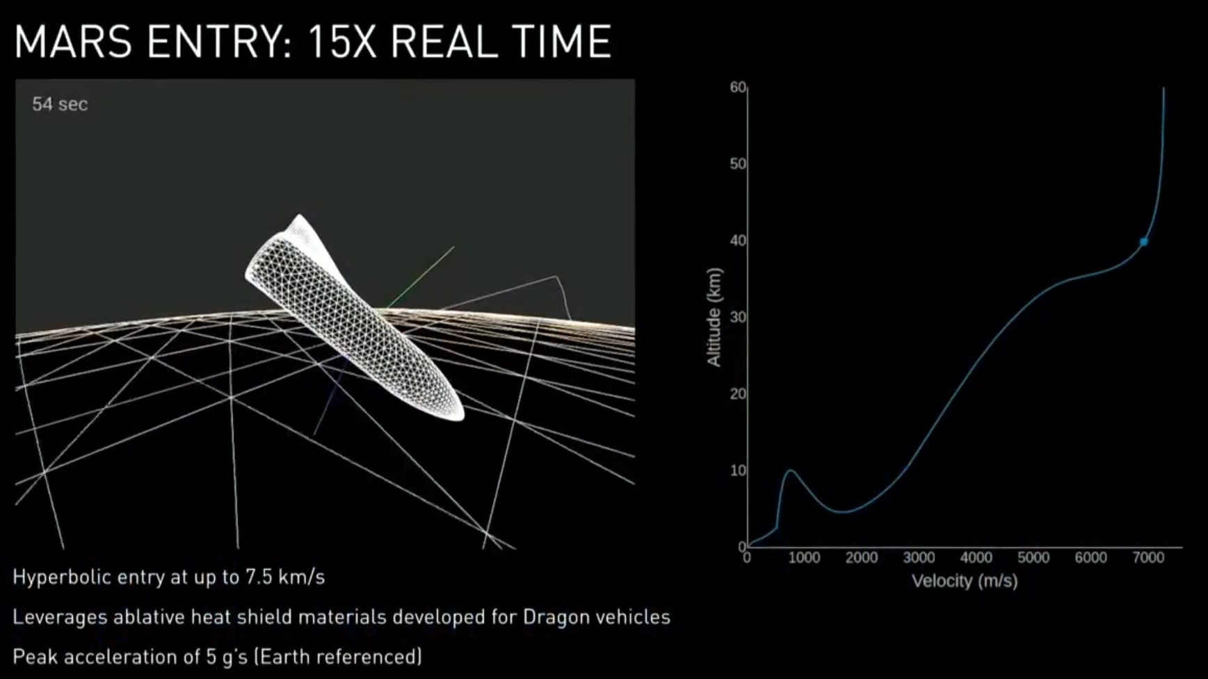(Expanded Image) In a 2017 Starship talk, Elon showed a simulated BFR Mars entry which I plotted my results against.

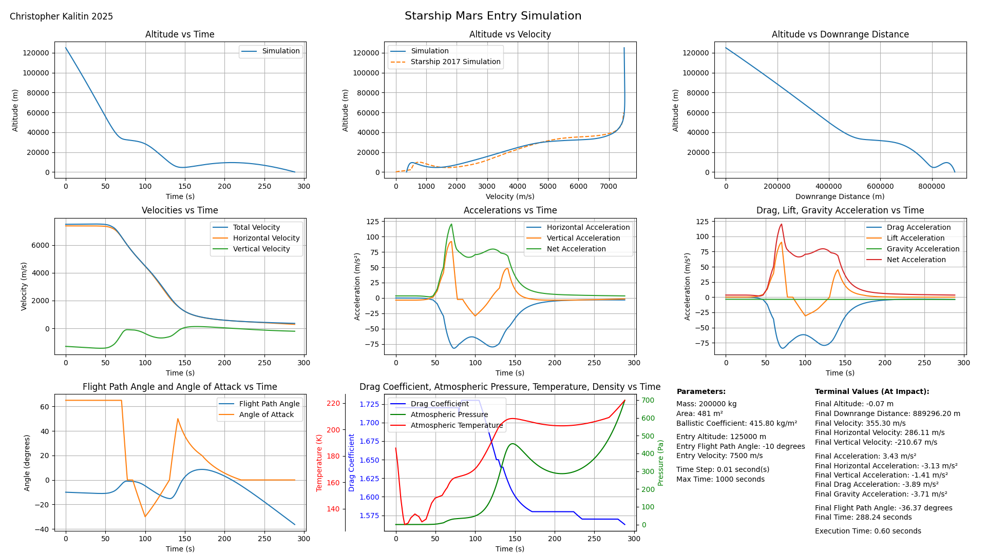
(Expanded Image) See the top middle chart for comparison between my Model and SpaceX’s higher fidelity simulation.

Just like the greater mass-to-area ratio (ballistic coefficient) of Opportunity vs. Perseverance, Starship has a much greater ballistic coefficient than either of them (~50 kg/m2, ~200 kg/m2, ~400 kg/m2, respectively). This means that Starship will require far more time in the atmosphere for drag to slow it down enough for a low propellant landing.

To fit to Starship using my model, I had to use a max angle of attack of 70 degrees (which corresponds to a Lift-to-drag ratio of ~1.2). This is getting to the point where angle of attack is not a useful model. This is stretching my model to its limits and we are veering away from reality.

However, I was able to get a good fit to SpaceX’s simulation. In the top middle chart, we see that Starship does what looks like two skips in the atmosphere before it reaches the surface. First, at ~40 km and second, at ~10km right before landing. I was able to replicate this in my model by varying the angle of attack over time (I encoded it at AoA vs. velocity).

Overall, throughout this modelling exercise I gained a far better appreciation for the importance of drag and lift in slowing down a vehicle during Martian atmospheric entry. For a vehicle like Starship, you want as much time in the atmosphere as possible, and if you were to follow a ballistic trajectory, you would not be able to land safely while using a reasonable amount of propellant.

Appendix 1: A Note on Blunt Body Aerodynamics

A blunt body (or bluff body) is defined as an object where pressure drag is the dominant drag force acting on it.

This is unlike a streamlined body, for which flow stays attached to the surface and friction drag dominates. For a streamlined body like an airfoil, pressure gradients develop at high angles of attack, which can lead to flow separation and stall. During stall, eddy formation in the wake causes pressure losses, which cause pressure drag. The normal operating condition of an airfoil is to have attached flow.

In contrast, because the purpose of a blunt body is to generate as much drag as possible, it always operates in a separated flow regime. The angle of attack can modulate the lift-to-drag ratio slightly, but it is not similar to an airfoil, where AoA is a much greater factor in determining lift and drag. Hence, the coefficient of drag, coefficient of lift, and lift-to-drag ratio can be used to simply model a blunt body vehicle.

Appendix 2: Finding Perseverance data vs. finding Tianwen-1 data

I wanted to model the entry of both Perseverance and Tianwen-1. When I looked online for Tianwen-1’s entry data, I found a publicly available paper within the first couple of results that fit my needs perfectly.

In contrast, it took me >30 minutes of searching every corner of the internet and finally resorting to asking ChatGPT to find me a (legal or illegal) way to get access to a particular paper that contained the data I needed.

Getting data on the Chinese Communist Party’s Mars lander was ~30x faster than getting data on the most recent and most advanced US Mars lander. WTF is this?? We cannot win like this.

NASA’s Technical Reports Server (NTRS) also gives me a 504 error every time I try to access it now. It worked for a day, and now I don’t have access. Did they rate limit me and not say? Seriously guys, are we trying to conquer the universe and give every human the ability to model Mars landers or not?

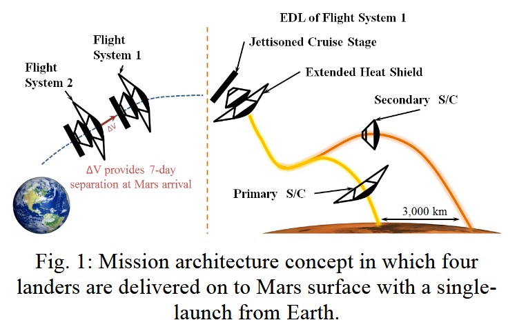
Appendix 3: Cool paper with a detachable heat shield Mars lander design

(Expanded Image)

While I was looking for historic Mars entry data, I found a cool paper that describes a Mars lander design with a detachable heat shield that contained several cool charts and insights that are applicable to Kerbal Space Program.

The entry vehicle contains two spacecraft, each with its own heat shield. During initial entry, both are attached on top of each other. Then, as the combined system descends to periapsis, the secondary (top) vehicle detaches and the primary (bottom) vehicle continues to descend. This way, two Mars rovers can be deployed at once to different locations on the surface.

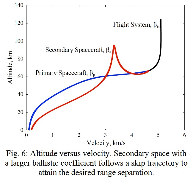
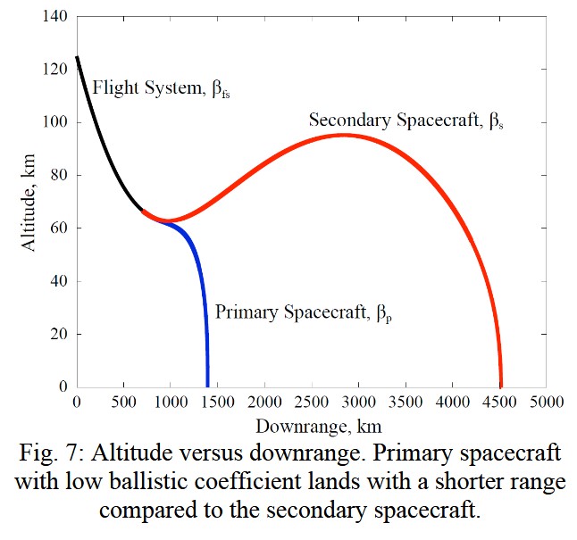
Because the primary vehicle has a larger surface area to mass ratio (ballistic coefficient) and because drag force is proportional to surface area, the primary vehicle decelerates faster than the secondary vehicle. This means the primary vehicle reaches the surface first and the secondary vehicle performs a skip off of Mars’ atmosphere and lands ~3000 km farther downrange.

This is the same phenomenon you can see in Kerbal Space Program when you decouple your heat shield after reentry but before you deploy parachutes, and it collides back into your craft. Because the heat shield itself has a greater ballistic coefficient than your capsule (without parachutes deployed), it decelerates faster than your capsule. Because the heat shield is below your capsule, it collides back into it.