Rewriting My Mars Entry Simulation Using Polar Coordinates
About two months ago I flew to SF and had the opportunity to speak to Casey Handmer while touring Impulse Labs. Handmer had previously done some Mars EDL modelling back when Starship was called the Interplanetary Transportation System, and I got some useful feedback on my Blunt Body Mars Entry Vehicle simulation from him. The most important piece of feedback was that modelling Mars as a flat surface is not an accurate approximation.
My old code is available when browsing the files associated with this commit. You can tell I wrote this code by hand due to the intrinsically human artisanal nature of the code. Handmade, no machine involvement, pure craftsmanship. (tl;dr code is shitty)
The Problem With A Flat Mars
Expanded Image
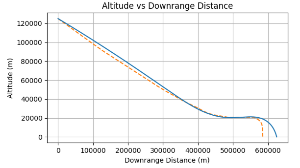
This shows a Y vs. X position plot from my original Mars simulation, modelling the planet as flat. This is a simulation of the Perseverance rover’s entry trajectory.
Expanded Image
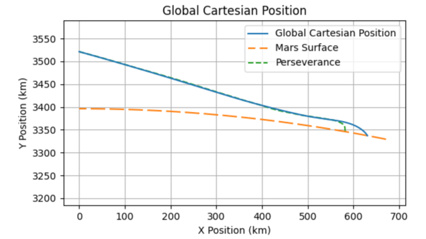
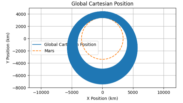
This shows a global Mars-center relative position plot from my updated simulation. Notice Mars curves down ~50 km from start to finish.
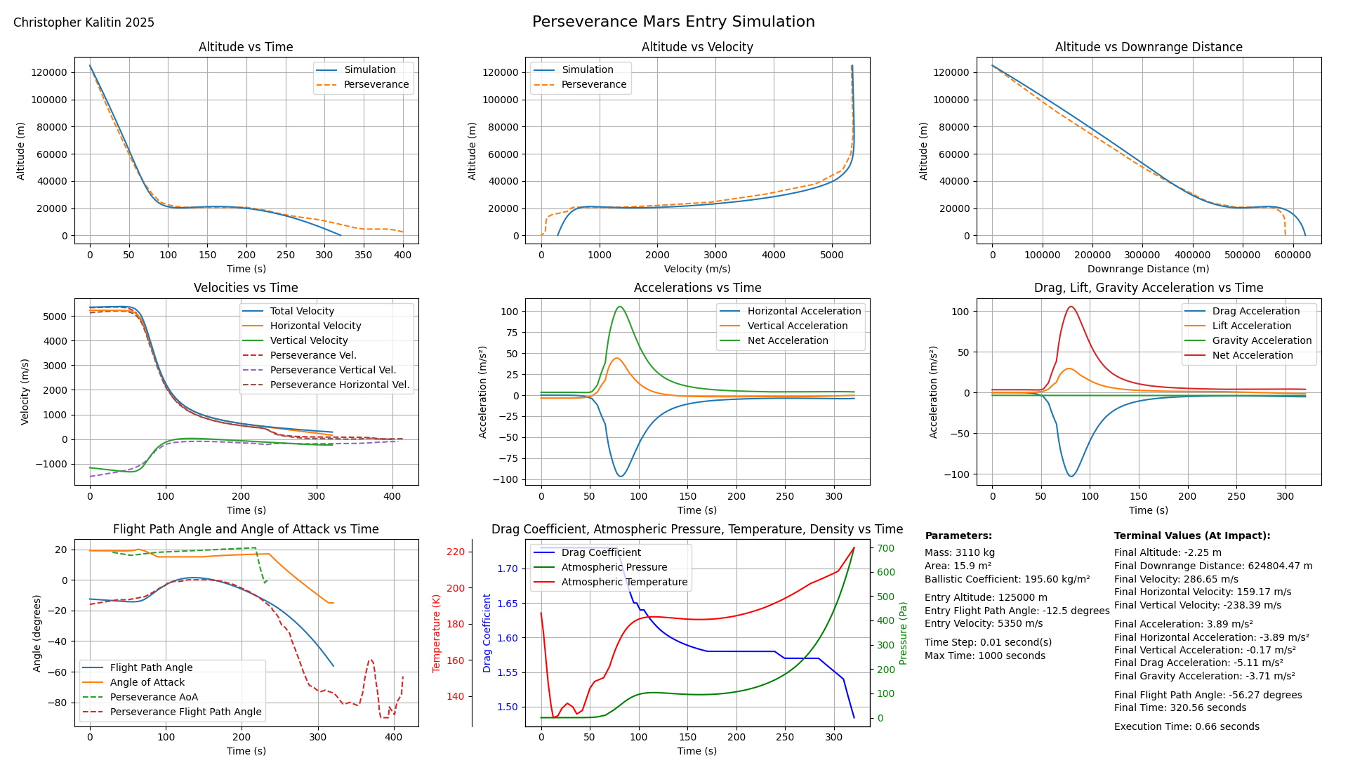
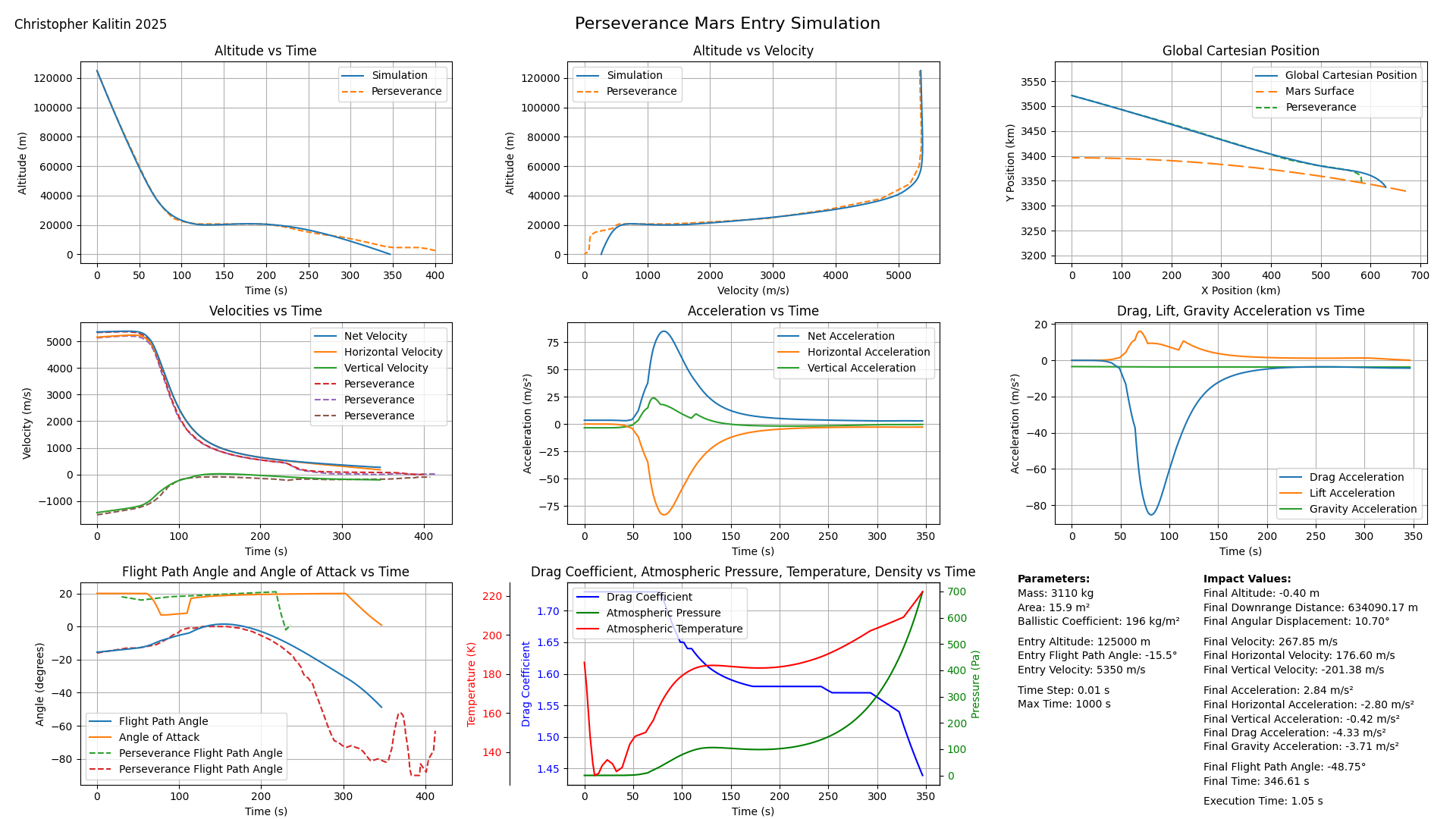
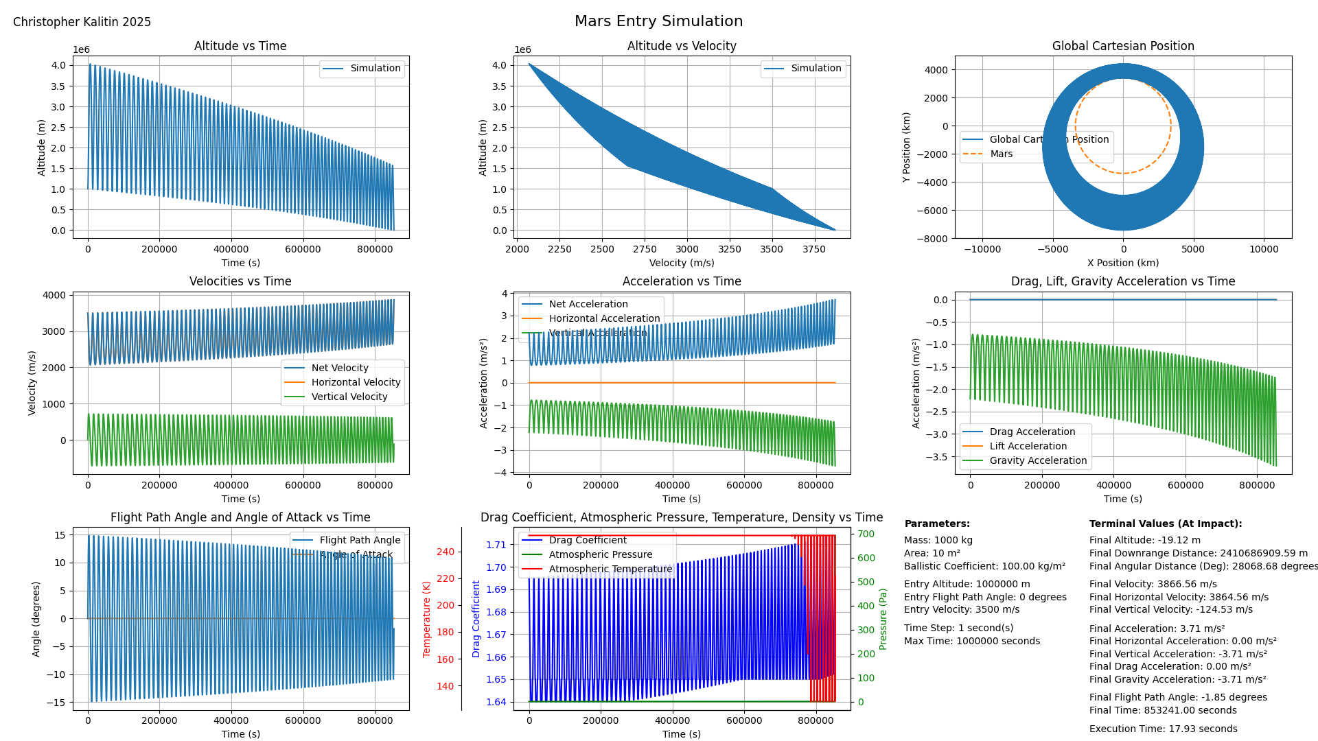
Above you can see two charts of a simulated entry of the Perseverance rover and a comparison to real data. The first chart is from my original flat Mars simulation, and the second is from my new polar-coordinate-based circular Mars simulation.
During entry, the Perseverance rover travels ~600 km along the surface of Mars. Mars has a radius of ~3,396 km, and using the angular displacement formula (Arc Length / Radius = Angular Displacement in Radians), we find that the planet curves down ~50 km during atmospheric entry. The initial condition of the simulation is at an altitude of 125 km, so the curvature of Mars is significant. In the flat Mars simulation, the rover’s downrange distance was 625 km, while in the polar-coordinate simulation it was 634 km.
Another limitation of the flat Mars approximation is that it cannot model an orbit around the planet. This becomes an issue when simulating high-velocity entries like Starship’s. During a 2016 SpaceX talk Elon shared a Starship Mars EDL simulation in which atmospheric entry occurs at ~7 km/s. Because the escape velocity of Mars is ~5.3 km/s, if Starship does not decelerate significantly during atmospheric entry, it will escape into deep space with no hope of returning to Mars. To remedy this, Starship begins reentry with a negative angle of attack, so that the lift vector is directed towards the planet. This both decelerates the vehicle and makes it spend more time in the atmosphere during reentry. Once the vehicle reaches ~5 km/s, it assumes a positive angle of attack to generate lift to delay landing, allowing for more atmospheric deceleration instead of propulsive deceleration.
My First Attempt
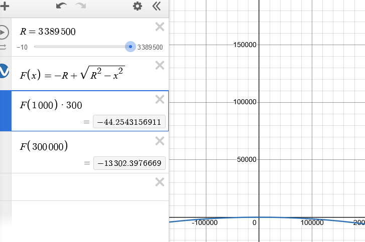
Notice that the equation for a circle is not linear (obviously). This means f(5x) != 5f(x), so the step size of the simulation changes how far you fall along the circle.
Originally I didn’t plan to fully rewrite all the simulation code because this was in service of another project in which I’ll simulate the entry of Stoke Nova’s upper stage into Earth’s atmosphere. So my first attempted solution was to simply increase the altitude of the vehicle every frame, effectively simulating the surface falling out from under you.
This approach didn’t work because a circular planet is not linear. I assumed that if in every frame I calculated how far Mars fell from under you and added this to the velocity, the net displacement of the surface would be equal regardless of the time step size.
However, because the equation of a circle is not linear, the step size of the simulation changes how far you fall along the circle on net. The screenshot of Desmos above shows that moving 300 km along the surface of Mars results in an altitude change of 13 km, while 300 steps of 1 km results in a net altitude change of 44 meters.
Polar Coordinates
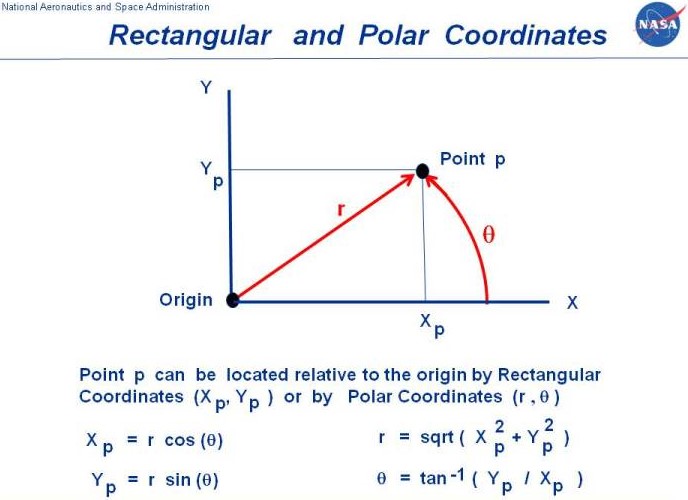
In case you don’t remember, polar coordinates consist of two variables: a radial distance and angular displacement (in radians). This allows you to describe your position relative to a center point—in this case, the center of Mars. The radial distance is the distance from the center of Mars to the vehicle (Mars radius + altitude), and the angular displacement is the angle between the positive Y axis and the vehicle’s position. My convention was that a positive angular displacement rotates the vehicle clockwise. (The standard convention is using the positive Y axis and rotating counterclockwise, but this made plotting easier in Matplotlib.)
I rewrote all the simulation code to use polar coordinates (and refactored my artisanal human code). However, without any further changes, this is just cartesian coordinates but with extra steps.
Consider the case of a vehicle 1000 km above the surface of a body of negligible gravity with 1 km/s horizontal velocity. In cartesian coordinates, the vehicle would travel horizontally 1 km every second, as expected. However, in polar coordinates, the vehicle would travel 1 km angularly every second, while maintaining a constant radial distance. This effectively means your vehicle is accelerating centripetally, which is not what we want.
So we must rotate the velocity vector every frame to align with the global Cartesian reference frame. In every step of the simulation, the angular distance in radians is calculated for the vehicle’s current radial distance. The velocity vectors are then rotated counterclockwise by this angle.
Expanded Image
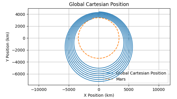
With globally consistent velocity vectors, an orbit around Mars can be simulated.
Expanded Image
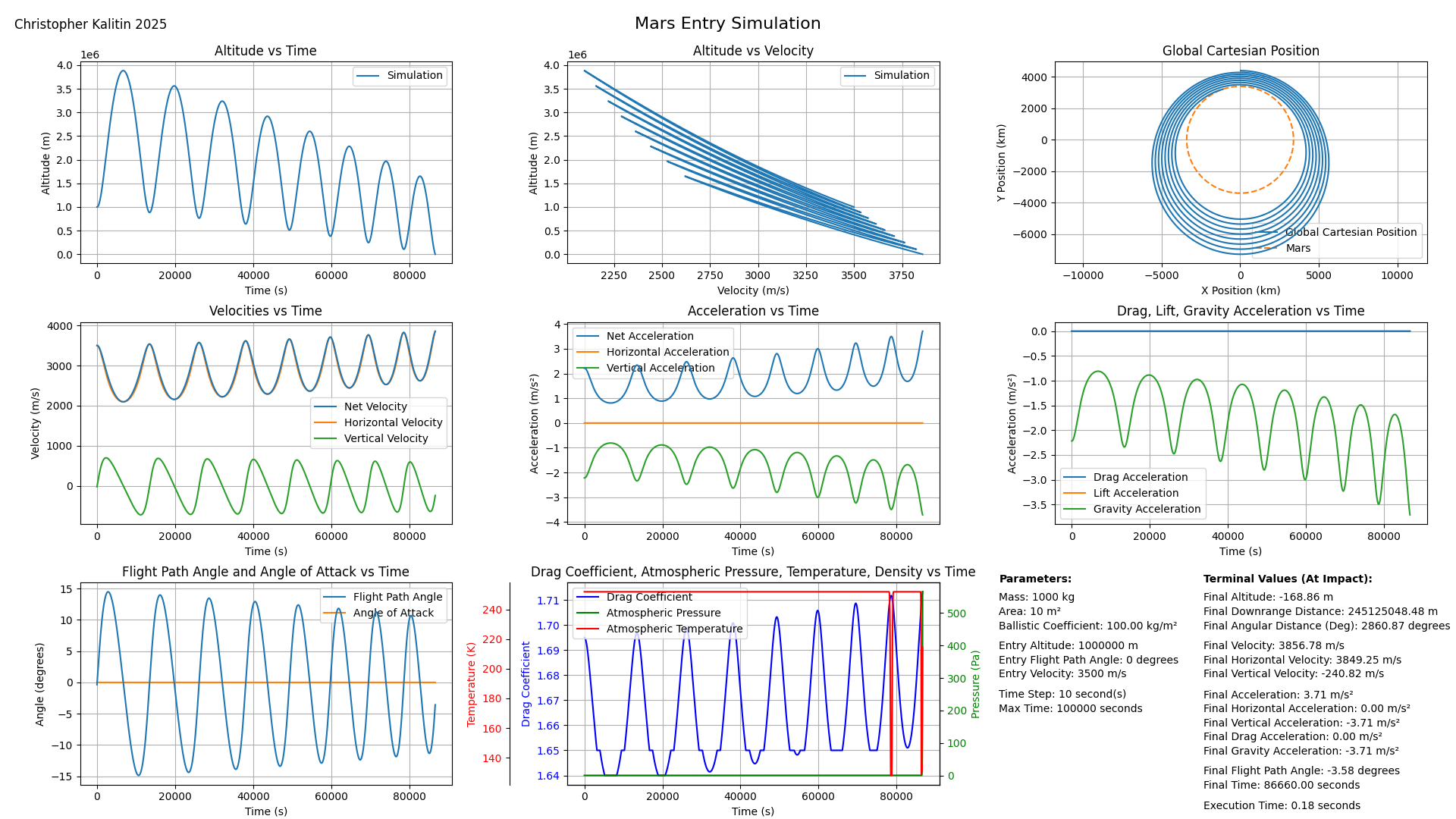
When changing the time step size from 10s to 1s, we notice that the vehicle stays in orbit for longer. Unexpected. Note that this simulation is with drag and lift forces disabled, so we expect it to be in orbit forever.
I next simulated an orbit around Mars with drag and lift forces disabled to ensure the simulation was operating correctly. You can see above that the vehicle was decelerating while orbiting around Mars, and that this deceleration increased with a larger time step size. My guess is that the vehicle’s velocity vector is being rotated at the wrong time or by a slightly too-large angle, resulting in part of the velocity vector being retrograde. At this point, the project was already sufficient for my purposes in my upcoming blog posts on modelling heat flux of Stoke Nova’s second stage during reentry and modelling ballistic coefficient vs. impact velocity. So I didn’t investigate that particular issue further.